xSIM

The simulation program logic is straightforward. The main code is a very compact function called xspde(). This calls xsim(), for the simulation, then xgraph() for the graphics. Most of the work is done by other specialized functions. Input parameters come from an input array, output is saved either in a data array, or else in a specified file. When completed, timing and error results are printed. In this chapter, we go into the workings of the simulation program, xsim.

How xSIM works

To summarize the previous chapters, xSIM will solve stochastic partial different equations for a vector field \(\boldsymbol{a}(t,\boldsymbol{x})\) and vector noise \(\boldsymbol{\zeta}(t,\boldsymbol{x})\), of form:

\[\frac{\partial}{\partial t}\boldsymbol{a}(t,\boldsymbol{x})=\mathbf{A}\left[\boldsymbol{a}\right]+\underline{\mathbf{B}}\left[\boldsymbol{a}\right]\cdot\boldsymbol{\zeta}(t,\boldsymbol{x})+\underline{\mathbf{L}}\left[\boldsymbol{\nabla}\right]\cdot\boldsymbol{a}\]

It can also solve ordinary stochastic equations, or partial differential equations without noise. Extensive error checking outputs are available. Both initial stochastic conditions and noise can have nonlocal spatial filters applied. All inputs are entered as part of an object-oriented structure. This includes the functions used to specify the equations and the quantities to average. The outputs can be either stored, or graphed interactively.

xSPDE includes a built-in multidimensional graphics tool, xGRAPH, treated in the next chapter.

Sequences

In many types of application, a sequence of stochastic equations requires simulation. In these cases the final field value after integration of one equation becomes the initial value of the next equation in the sequence. At the end of each simulation loop, global averages and error-bars are calculated and stored for output.

Sequences therefore are the basic concept used in both the input of parameters to xSPDE, and the storage of data generated.

Input and data arrays

To explain xSIM in full detail,

• Simulation inputs are stored in the input cell array.
• This describes a sequence of simulations, so that input = {in1, in2, ...}.
• Each structure in describes a simulation, whose output fields are the input of the next.
• The main function is called using [error, input, data, rawdata] = xsim([rawdata,] input).
• Averages are recorded sequentially in the data cell array.
• Raw trajectory data is stored in the raw cell array if required.

The sequence input has a number of individual simulation objects in. Each includes parameters that specify the simulation, with functions that give the equations and observables. If there is only one simulation, just one individual specification in is needed. All outputs can be saved to disk storage if required.

The optional [data,] input is only used when there is previous raw data that needs analysis. If this is present, no new simulation takes place. Any observe functions in the new input will be employed to take further averages over the existing raw data. This allows re-analysis of large simulation data-sets without more simulations.

The returned error is a vector: the first component is the maximum error found, the second component is the elapsed time. The returned input structure is available to the user to give the data file-name, in case xSIM needs to store data with a new file-name. For data security, it will not overwrite existing data.

If xSIM is called within xSPDE, it will generate graphs with its own graphics program xGRAPH. Otherwise, data can be stored then graphed later using xGRAPH.

Customization options

There are a wide range of customization options available for those who wish to have the very own xSIM version.

Customization options include functions the allow user definition of:

• inputs
• interfaces
• stochastic equations
• mean observables
• linear propagators
• coordinate grids
• noise correlations
• integration methods

There are four internal options for stochastic integration methods, but arbitrary user specification is also possible.

User-defined functions have to return specified array sizes, compatible with the internal arrays in xSIM. These sizes are checked by xSIM prior to a simulation. The xSIM program will print out a record of its progress.

Averaged data

Observables and functions

To allow options for taking averages, these are carried out in two stages. The first type of average is a local average, taken over any function of the locally stored ensemble of trajectories. These use the :func:observe functions, specified by the user. The default is the real values of each of the fields, stored as a vector. Multiple observe functions can be used, and they are defined as a cell array of functions.

Next, any function can be taken of these local averages, using the :func:function transformations, again specified by the user. The default is the original set of local averages. This is useful if different combinations, such as normalised ratios are needed, or to combine the averages at different times. These second level function outputs are then averaged again over a second level of ensemble averaging, if specified. This is used to obtain estimates of sampling and step-size errors in the final data outputs.

This is explained below in more detail.

Observe functions

During the calculation, observables are calculated and averaged over the ensembles(1) parallel trajectories in the xpath() function. These are determined by the functions in the observe() cell array.

The number of observe() functions may be smaller or larger than the number of vector fields. The observable may be a scalar or vector. These include the averages over the ensembles, and can be visualized as a single graph with one or more lines. The observe() functions use for input and output the flat or matrix type internal arrays.

Next, arbitrary functional transforms can be taken, using the function cell array. These functions can use as their input the full set of observe() output data cell arrays, including a time index. They default to the original observe() data if they are not user-defined. Functional transforms are most useful if one wishes to use functions which require knowledge of normalization or ensemble averages of lower-level data. There can be more function definitions than observe() functions if needed.

Each observe() function or transformation in xsim() defines a single logical graph for the simulation output. However, the graphics function xgraph() can generate several projections or views of the same dataset, as explained below.

Combined observables: data

These results are added to the earlier results in the cell array data, to create a combined set of graphs for the simulation. Initially, both the first and second moment is stored, in order to allow calculation of the sampling error in each quantity. These are averaged over the higher level ensembles, to allow estimates of sampling errors. Each resulting graph or average data is each stored in an array of size

data - all graphics datasets from one sequence member collected in a cell array

Cell Array, has dimension: data{graphs}, made up of a collection of arrays:

1. graph: observable or function making up a single graph

   Array, has dimension: (components, errorchecks, in.points).

In the simplest case, there is just one vector component per average. More generally, the number of components is larger than this if there is a requirement to compare different lines in one graph. Note that, unlike the propagating field, the time dimension is fully expanded. This is necessary in order to generate outputs at each of the in.points(1) time slices.

When step-size checking is turned on using the checks flag set to 1, a low resolution field is stored for comparison with a high-resolution field of half the step-size, to obtain the time-step error. The observables which are stored have three check indices which are all included in the array. These are the high resolution means, together with error-bars due to time-steps, and estimates of high-resolution standard deviations due to sampling statistics.

The second dimension, errorchecks, is the total number of components in the data array due to error-checking. After ensemble averaging, the second index is typically c = 1, 2, 3, which is used to index over the:

1. mean value,
2. time-step error-bars and
3. sampling errors

respectively for each space-time point and each graphed function. As a result, the output data ready for graphing with xGRAPH includes step-size error bars and plotted lines for the two estimated upper and lower standard deviations, obtained from the statistical moments.

Stochastic flowchart

The main program logic is nearly self-explanatory. It has four functions and two main arrays that store results.

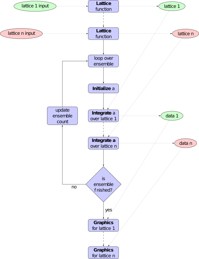
Fig. 30 xSPDE flowchart, showing the data, lattice and field processing.

There are also two important computational routines behind the scenes, which need to be kept in mind. These are da(), which is short for difference in \(a\). This is completely user specified, and gives a local step in time. The next workhorse routine is xprop(). This is not a beefy Rugby forward, but calculates spatial propagation.

The logical order is as follows:

xsim() decides the overall workflow, and parallel operation at a high level. Here, in.ensembles(3) is used to specify parallel integration, with a parfor loop. The random seeds include data from the loop index to make sure the noise is independent for each ensemble member, including parallel ensembles.

xinpreferences()

is called by xlattice() to set the defaults that are not already entered.

xlattice()

creates a space-time lattice from the input data, which is a data-structure. This also initializes the actual data array for averaging purposes. Next, a loop is initiated over an ensemble of fields for checking and ensemble averaging. The calculations inside the loop can all be carried our in parallel, if necessary. These internal steps are actually relatively simple.

xensemble()

repeats each stochastic path for the check/ensemble loop. It is important to notice that the random seed is reset at the start of each ensemble loop. The seed has a unique value that is different for each ensemble member. Note that for successive simulations that are not stored in the same data array, the seed should ideally be manually chosen differently for inputs to successive integration blocks, in order to guarantee independent noise sequences. The check variable can be set to in.checks = 0,1. The integration is executed once with in.checks = 0. With in.checks = 1, there is another error-checking integration, using half the step-size the second time. This takes three times as long overall. The matrices used to define the interaction picture transformations are stored for each check loop, as they vary with step-size.

xpath()

propagates the field a over a path in time. There are steps time-steps for each point stored in time, to allow for greater accuracy without excessive data storage, where needed. This integrates the equations for a predetermined time duration. Note that the random seed has the same value for both the check loops. This is because the same number of random variates must be generated in the same order to allow accurate extrapolation. The two loops must use the same random numbers, or else the check is not accurate. For random numbers generated during the integration, the coarse step will add two fine step random noises together, to achieve the goal of identical noise behavior. Results of any required averages, variances and checks are accumulated in the data array.

xprop()

uses either Fourier space or finite differences to calculate a step in the interaction picture, using linear transformations that are pre-calculated. There are both linear transformations and momentum dependent terms available. These are pre-calculated by the xlattice() function, and stored in the prop arrays.

Simulation user functions

initial()

is used to initialize each integration in time. This is a user-defined function, which can involve random numbers if there is an initial probability distribution. This creates a stochastic field on the lattice, called a. Initialization functions can use coordinates, r.t,``r.x``, r.y, r.z, or for larger dimensions, using numerical lattice labels r.x{1}, r.x{2}, r.x{3}, r.x{4}. Numerical labels can be used for any number of dimension if the switch numberaxis=1. The default is xinitial(), which sets fields to zero.

step()

is the algorithm or method computes each space-time point in the lattice. This also generates the random numbers fields at each time-step. It can be user-modified by setting the handle in.step. The default is in.step = xRK4.

observe()

is a cell array of observation functions whose output is averaged over the ensembles, called from xpath(). In general, this returns an array whose first coordinate is the line-number of the n-th graph. The default, xobserve(), returns the real amplitudes. The return value is averaged over the local ensemble and stored as data, d{n}. Note that the input of observe() is the complete field array.

function()

is a cell array of functions used when graphs are needed that are functions of the observed averages. The default value is simply d{n}. This is further averaged over higher ensembles to obtain sampling error estimates. Note that the input of function() is the complete data cell array, d, which includes all the space-time averages for all the observe functions available.

linear()

is the linear response, including transverse derivatives in space. The default, xlinear(), sets this to zero. Derivatives are specified using arrays r.Dx, r.Dy, r.Dz, or for larger dimensions, using numerical lattice labels r.D{2}, r.D{3}, r.D{4}, r.D{5}.

da()

is called by step() to calculate derivatives at every step in the process, including the stochastic terms. Returns a vector with in.fields(1) first components.

define()

is called by step() to calculate auxiliary fields at every step in the process. Returns a vector with in.fields(2) first components.

Details of the different parts of the program are given below. Note that the functions tic() and toc() are called to time each simulation.

The xSPDE data and arrays that are user accessible are parameters r, fields a, average observables data, and raw trajectories rawdata. Apart from the parameters, which are Matlab structures, all fields and data are arrays.

Data arrays and ensembles

There is a unified index model in all xSPDE arrays. However, in the internal calculations of derivatives and observables, these indices are flattened to give a matrix, as explained below. In all cases, the underlying xSPDE array index ordering is kept exactly the same:

1. field index \(i\)
2. ensemble or error-checking index \(e\) or \(c\)
3. time, t index \(j_1\)
4. x index \(j_2\)
5. y index \(j_3\)
6. z index \(j_4\) ..

The number of space dimensions is arbitrary. To conserve storage, one time - the current one - is stored for propagating fields. The ensemble index can be adjusted to increase or decrease local memory usage. If needed, all data generated can be saved in rawdata arrays.

The fields a are complex arrays stored discretely on space or momentum grids. Internally, the fields are matrices stored on the flattened xSPDE internal lattice, with just two indices only. Transformations to Fourier space are used both for interaction picture propagation [Caradoc-Davies2000] and for averages over Fourier space.

Two different types of Fourier representations are used. In xsim, Fourier transformations are for propagation, which requires the fastest possible methods, and uses \(k=0\) as the first or lowest index. In xgraph, Fourier transformations are for graphical representations. Hence, the indices are re-ordered to a conventional index ordering, with negative momentum values in the first index position.

The parameters are stored in a structure called, simply, r. It is available to all user-definable routines. The label r is chosen because the parameters include the grid coordinates in space and time. These structures reside in a static internal cell array that combines both input and lattice parameters, including the interaction picture transformations, called latt. The data in latt is different for each simulation in a sequence.

Averaged results are called observables in xSPDE. For each sequence, these are stored in either space or Fourier domains, in the array data, as determined by the transforms vector for each observable. This is a vector of switches for each of the space-time coordinates. The data arrays obtained in the program as calculations progress are stored in cell arrays, cdata, indexed by a sequence index.

If required, rawdata ensemble data consisting of all the trajectories a developing in time can be stored and output. This is memory intensive, and is only done if the raw option is set to 1.

All calculated data, including fields, observables and graphics results, is stored in arrays of implicit or explicit rank (2+d), where d is the space-time dimension given in the input. The first index is a field index \((i)\), the second a statistics/errors index \((e)\), while the remaining indices \(j\equiv j_{1},\ldots j_{d}\equiv j_{1},\mathbf{j}\) are for time and space. The space-time dimension d is unlimited.

xSPDE flattened arrays

When the fields, noises or coordinates are integrated by the xSPDE integration functions, they are flattened to a matrix. The first index is the field index, and the combined second index covers all the rest. It is more convenient when calculating derivatives and observables in xSIM, to use these flattened arrays or matrices. They are obtained by combining indices \((e,j)\) into a flattened second index \(J\). This is faster and more compact notationally. Hence, when used in xSPDE functions, the fields are indexed as \(a(i,J)\).

xSPDE array types

There are several different types of arrays used. These are as follows:

• Field arrays, \(a(i,e_1,1,\mathbf{j})\) - these have an ensemble index of up to \(e_1=ensembles(1)\), but just a single point in time for efficiency. The fields are flattened to give \(a(i,J)\).
• Random and noise arrays, \(w(n,e_1,1,\mathbf{j})\) - these are like field arrays, except that they contain random numbers for the stochastic equations. Random and noise fields are flattened to give \(w(n,J)\), where n ranges over the available number of noise variables.
• Coordinate arrays \(r.x\{l\}(1,e_1,1,\mathbf{j})\) - these store the values of coordinates at grid-points, depending on the axis \(l=2,\ldots d\) , and are part of the main internal data structure, r. These only have a single first index. Coordinates are flattened to give \(r.x\{l\}(1,J)\). For less than four total dimensions, this notation is replaced by \(r.t\),:math:r.x(1,J),:math:r.y(1,J),:math:r.z(1,J). There is a similar array in momentum space, \(k\{l\}(1,J)\).
• Raw arrays, \(r\{s,c,e_2\}(i,e_1,j)\) - like fields, but with all points stored. Use with care, as they take up large amounts of memory! Here, we use the notation that \(j=j_1,j_2,\ldots j_d\) for \(d\) space-time dimensions. Note that when output or saved, these have additional cell indices: \(s=1,\ldots S\) is the sequence number, \(c=1,2\) for the error-checking of the time-step \(e_2=1,2\) for the combined serial and parallel ensemble index. To keep track of all the data, an error-check and two ensemble indices are needed here.
• Data arrays, \(d\{n\}(i,c,j)\) - these store the averages, or arbitrary functions of them, with an error-checking index \(c=1,2,3\), to store checking data at all time points. No ensemble index is needed, as these are ensemble averages, so the second index is used to store the checking data at this stage in the code. Here \(j=j_1,j_2,\ldots j_d\) space-time points. Next, if the data is transformed, the \(j\) index gives the index in Fourier space-time, as indicated by the transforms flag.
• Graphics arrays, \(g\{n\}(i,c,j)\) - these store the data that is actually plotted, and can include further functional transformations if required.

The first or field index \(i\) in a graphics or data array describes different lines on a graph. There can be different first dimensions between fields, noises and output data, as they are specified using different parameters. For only a single output graph, the cell index is not needed.

All outputs have an extra high-level cell index \(\{n\}\) called the graph or function index. This corresponds to the index \(\{n\}\) of the observe function used to generate averages. One can have several data arrays in a larger cell arrays to make a number of distinct output graphs labelled \(n\), each with multiple averages. Sequences generate separate graphics arrays in sequence.

More details of ensembles, grids and the internal lattice are given below. Note that the term lattice is used to refer to the total internal field storage. This combines the local ensemble and the spatial grid together.

Ensembles

Ensembles are used for averaging over stochastic trajectories. They come in three layers: local, serial and parallel, in order to optimize simulations for memory and for parallel operations. The in.ensembles(1) local trajectories are used for array-based parallel ensemble averaging, indexed by \(e_1\). These trajectories are stored in one array, to allow fast on-chip parallel processing.

Distinct stochastic trajectories are also organized at a higher level into a set of in.ensembles(2) serial ensembles for statistical purposes, which allows a more precise estimate of sampling error bars. For greater speed, these can be integrated using in.ensembles(3) parallel threads. In raw data, these are combined and indexed by the \(e_2\) cell index.

This hierarchical organization allows allows flexibility in allocating memory and optimizing parallel processing. It is usually faster to have larger values of in.ensembles(1), but more memory intensive. Using larger values of in.ensembles(2) is slower, but requires less memory. Using larger values of in.ensembles(3) is fast, but requires the Matlab parallel toolbox, and uses both threads and memory resources. It is generally not effective to increase in.ensembles(3) above the maximum number of available computational cores.

In summary, the stochastic ensembles are defined as follows:

1. Local ensemble: The first or local ensemble contains ensembles(1) trajectories stored on the xSPDE internal lattice and processed using matrix operations. These are averaged using vector instructions, and indexed locally with the \(e_1\) index.
2. Serial ensemble: The second or serial ensemble contains ensembles(2) of the local ensembles, processed in a sequence to conserve memory.
3. Parallel ensemble: The third or parallel ensemble contains ensembles(3) of the serial ensembles processed in parallel using different threads to allow multi-core and multi-CPU parallel operations. The serial and parallel ensembles are logically equivalent, and give identical results. They are indexed by the combined \(e_2\) cell index in raw data.

Coordinates, integrals and derivatives

Time and space

The default space-time grid

for plotted output data is rectangular, with

dx(i) = in.ranges(i) / (in.points(i) + in.boundaries(i))

The time index is 1, and the space index i ranges from 2 to dimension. The maximum space-time dimension is in.dimension = 4, while in.ranges(i) is the time and space duration of the simulation, and in.points(i) is the total number of plotted points in the i-th direction. The input in.boundaries=-1,0,1 changes the lattice locations and steps to the most suitable for the given type of space boundary. The offsets are -1 for Neumann or vanishing derivative boundaries (also used for time), 0 for periodic boundaries (the default value) and 1 for Dirichlet or vanishing field boundaries.

Time is advanced in basic integration steps that are equal to or smaller than dx(1), for purposes of controlling and reducing errors:

dt = dx(1) / (in.steps * nc)

Here, steps is the minimum number of steps used per plotted point, and nc = 1, 2 is the check number. If nc = 1, the run uses coarse time-divisions. If nc = 2 the steps are halved in size for error-checking. Error-checking can be turned off if not required.

The xSPDE space and momentum grid can have any dimension, provided there is enough memory. However, default label values are limited to ten. Using more than six to ten total dimensions causes large time and storage requirements and is usually not very practical.

Space grid

We define the grid cell size \(dx_{j}\) in the \(j\)-th dimension in terms of maximum range \(r_{j}\), the number of points \(n_{j}:\), and the boundary value \(r_{j}\), as:

\[dx_{j}=\frac{r_{j}}{n_{j}+b_{j}}.\]

Each grid starts at a value defined by the vector origin. Using the default values, the time grid starts at \(t=0\) and ends at \(t=T=r_{1}\), for \(n=1,\ldots N_{j}\):

\[t\left(n\right)=(n-1)dt.\]

Unless there is an offset origin , the \(j\)-th coordinate grid starts at \(-r_{j}/2\) and ends at \(r_{j}/2\) , so that, for \(n=1,\ldots n_{j}\):

\[x_{j}\left(n\right)=-r_{j}/2+(n-1)dx_{j}.\]

Momentum grid

All fields can be transformed into Fourier space for taking averages in the observe() function. This is achieved with the user-defined transforms cell array. This is a cell array of vector switches. For any graph and dimension where transforms is set to unity, the corresponding Fourier transform is taken.

The momentum space graphs and spectral methods all use a Fourier transform definition so that, for \(d\) dimensions:

\[\tilde{\boldsymbol{a}}\left(\boldsymbol{k},\omega\right)=\frac{1}{\left(2\pi\right)^{d/2}}\int d\boldsymbol{x}e^{i(\omega t-\boldsymbol{k}\cdot\boldsymbol{x})}\boldsymbol{a}\left(\boldsymbol{x},t\right)\]

In order to match this to the standard definition of a discrete FFT, the \(j\)-th momentum lattice cell size \(dk_{j}\) in the \(j\)-th dimension is defined in terms of the number of points \(N_{j}:\)

\[dk_{j}=\frac{2\pi}{dx_{j}N_{j}}.\]

The momentum range is therefore

\[K_{j}=\left(N_{j}-1\right)dk_{j},\]

while the momentum lattice starts at \(-K_{j}/2\) and ends at \(K_{j}/2\) , so that when graphing the data:

\[k_{j}\left(n\right)=-K_{j}/2+(j-1)dk_{j}.\]

However, due to the standard definitions of discrete Fourier transforms, the order used during computation and stored in the data arrays is different, namely:

\[k_{j}\left(n\right)=0..(N_{j}-1)/2)dk_{j},-(N_{j}-1)/2)dk_{j},.-dk_{j}\]

Averages

There are functions available in xSPDE for grid averages, spatial integrals and derivatives to handle the spatial grid. These can be used to calculate observables for plotting, but are also available for calculating stochastic derivatives as part of the stochastic equation. They operate in parallel over the local ensemble and lattice dimensions. They take a vector or scalar quantity, for example a single field component, and return an average, a space integral, and a spatial derivative respectively. In each case the first argument is the field, the second argument is a vector defining the type of operation, and the last argument is the parameter structure, r. If there are only two arguments, the operation vector is replaced by its default value.

Spatial grid averages can be used to obtain stochastic results with reduced sampling errors if the overall grid is homogeneous. An average is carried out using the builtin xSPDE function xave() with arguments (o, [av, ] r).

This takes a vector or scalar field or observable, for example o = [1, n.lattice], defined on the xSPDE local lattice, and returns an average over the spatial lattice with the same dimension. The input is a field or observable o, and an optional averaging switch av. If av(j) > 0, an average is taken over dimension j. Space dimensions are labelled from j = 2 ... 4 as elsewhere. If the av vector is omitted, the average is taken over all space directions. To average over the local ensemble and all space dimensions, use xave(o). Averages are returned at all lattice locations.

Higher dimensional graphs of grid averages are generally not useful, as they are simply flat. The xSPDE program allows the user to remove unwanted higher dimensional graphs of average variables. This is achieved by setting the corresponding element of pdimension to the highest dimension required, which depends on which dimensions are averaged.

For example, to average over the entire ensemble plus space lattice and indicate that only time-dependent graphs are required, set av = in.dx and:

in.pdimension = 1

Note that xave() on its own gives identical results to those calculated in the observe() functions. Its utility comes when more complex combinations or functions of ensemble averages are required. If the transforms switch is set, then momentum space averages are returned.

Integrals

Integrals over the spatial grid allow calculation of conserved or other global quantities. To take an integral over the spatial grid, use the xSPDE function xint() with arguments (o, [dx, ] r).

This function takes a scalar or vector quantity o, and returns a trapezoidal space integral over selected dimensions with vector measure dx. If dx(j) > 0 an integral is taken over dimension j. Dimensions are labelled from j = 1, ... as in all xSPDE standards. Time integrals are ignored at present. Integrals are returned at all lattice locations. To integrate over an entire lattice, set dx = r.dx, otherwise set dx(j) = r.dx(j) for selected dimensions j.

As with averages, the xSPDE program allows the user to remove unwanted higher dimensional graphs when the integrated variable is used as an observable. For example, in a four dimensional simulation with integrals taken over the \(y\) and \(z\) coordinates, only \(t\)- and \(x\)-dependent graphs are required. Hence, set dx to [0, 0, r.dx(3), r.dx(4)], and:

in.pdimension = 2

If momentum-space integrals are needed, use the transforms switch to make sure that the field is Fourier transformed, and input dk instead of dx. Note that xint() returns a lattice observable, as required when used in the observe() function. If the integral is used in another function, note that it returns a matrix of dimension [1, lattice].

Derivatives in equations

xSPDE can support either spectral or finite difference methods for derivatives. The default spectral method used is a discrete Fourier transform, but other methods can be added, as the code is inherently extensible. These derivatives are obtained through function calls.

The code to take a spectral derivative, using spatial Fourier transforms, is carried out using the xSPDE xd() function with arguments (o, [D, ] r). This can be used both in calculating derivatives for equations, and for averages or observables if they are needed.

This function takes a scalar or vector quantity o, and returns a spectral derivative over selected dimensions with a derivative D, by Fourier transforming the data. Set D = r.Dx for a first order x-derivative, D = r.Dy for a first order y-derivative, and similarly D = r.Dz.*r.Dy for a cross-derivative in z and y. Higher derivatives require powers of these, for example D = r.Dz.^4`. For higher dimensions use numerical labels, where D = r.Dx becomes D = r.D{2}, and so on. Time derivatives are ignored at present. Derivatives are returned at all lattice locations.

If the derivative D is omitted, a first order x-derivative is returned. Note that xd() returns a lattice observable, as required when used in the observe() function. If the integral is used in another function, it returns a matrix of dimension [1, lattice].

Finite difference first derivatives

The code to take a first order spatial derivative with finite difference methods is carried out using the xSPDE function xd1() with arguments (o, [dir, ] r).

This takes a scalar or vector o, and returns a first derivative with an axis direction dir. Set dir = 2 for an x-derivative, dir = 3 for a y-derivative. Time derivatives are ignored at present. Derivatives are returned at all lattice locations.

If the direction dir is omitted, an x-derivative is returned. These derivatives can be used both in calculating propagation, and in calculating observables. The boundary condition is set by the in.boundaries input. It can be made periodic, which is the default, or Neumann with zero derivative, or Dirichlet with zero field.

Finite difference second derivatives

The code to take a second order spatial derivative with finite difference methods is carried out using the xSPDE xd2() with arguments (o, [dir, ] r) function.

This takes a scalar or vector o, and returns the second derivative in axis direction dir. Set dir = 2 for an x-derivative, dir = 3 for a y-derivative. All other properties are exactly the same as xd1().

Interaction picture and Fourier transforms

The xSPDE algorithms all allow the use of a sequence of interaction pictures. Each successive interaction picture is referenced to \(t=t_{n}\), for the n-th step starting at \(t=t_{n}\), so \(\boldsymbol{a}_{I}(t_{n})=\boldsymbol{a}(t_{n})\equiv\boldsymbol{a}_{n}\). It is possible to solve stochastic partial differential equations in xSPDE using explicit derivatives, but this is often less efficient.

A conventional discrete Fourier transform (DFT) using a fast Fourier transform method is employed for the interaction picture (IP) transformations used in computations, as this is fast and simple. In one dimension, this is given by a sum over indices starting with zero, rather than the Matlab convention of one. Hence, if \(\tilde{m}=m-1\):

\[A_{\tilde{n}}=\mathcal{F}\left(a\right)=\sum_{\tilde{m}=0}^{N-1}a_{\tilde{m}}\exp\left[-2\pi i\tilde{m}\tilde{n}/N\right]\]

Suppose the spatial grid spacing is \(dx\), and the number of grid points is \(N\), then the maximum range from the first to last point is:

\[R=(N-1)dx\]

We note that the momentum grid spacing is

\[dk=\frac{2\pi}{Ndx}\]

The IP Fourier transform can be written in terms of an FFT as

\[\boldsymbol{A}\left(\boldsymbol{k}_{\boldsymbol{n}}\right)=\prod_{j}\left[\sum_{\tilde{m}_{j}}\exp\left[-i\left(dk_{j}dx_{j}\right)\tilde{m}_{j}\tilde{n}_{j}\right]\right]\]

The inverse FFT Fourier transforms automatically divide by the correct factors of \(\prod_{j}N_{j}\) to ensure invertibility. Note also that due to the periodicity of the exponential function, negative momenta are obtained if we consider an ordered lattice such that:

\[\begin{split}\begin{aligned} k_{j} & = (j-1)dk\,\,\,(j\le N/2)\\ k_{j} & = (j-1-N)dk\,\,(j>N/2) \end{aligned}\end{split}\]

This Fourier transform is multiplied by an appropriate factor to propagate in the interaction picture, than an inverse Fourier transform is applied. While it is for interaction picture transforms, an additional scaling factor is applied to obtain transformed fields in averages.

In other words, in the averages

\[\tilde{a}_{n} = \frac{dt}{\sqrt{2\pi}} A_{\tilde{n}'}\]

where the indexing change indicates that graphed momenta are stored from negative to positive values. Note also that for frequency spectra a positive sign is used in the frequency exponent, to agree with physics conventions.

Interaction picture derivatives

For calculating derivatives in the interaction picture, the notation \(D\) indicates a derivative. To explain, one integrates by parts:

\[D^{p}\tilde{\boldsymbol{a}}\left(\boldsymbol{k}\right)=\left[ik_{x}\right]^{p}\tilde{\boldsymbol{a}}\left(\boldsymbol{k}\right)=\frac{1}{\left(2\pi\right)^{d/2}}\int d\boldsymbol{x}e^{-i\boldsymbol{k}\cdot\boldsymbol{x}}\left[\frac{\partial}{\partial x}\right]^{p}\boldsymbol{a}\left(\boldsymbol{x}\right)\label{eq:Fourier derivative}\]

This means, for example, that to calculate a one dimensional space derivative in the Linear interaction picture routine, one uses:

• \(\nabla_{x}\rightarrow\) r.Dx

Here r.Dx returns an array of momenta in cyclic order in dimension \(d\) as defined above, suitable for an FFT calculation. The imaginary \(i\) is not needed to give the correct sign, from the equation above. Instead, it is included in the D array. In two dimensions, the code to return a full two-dimensional Laplacian is:

• \(\boldsymbol{\nabla}^{2}=\nabla_{x}^{2}+\nabla_{y}^{2}\rightarrow\) r.Dx.^2+r.Dy.^2

Note that the dot in the notation of .^ is needed to take the square of each element in the array.

Spectra in the time-domain

For calculating a spectrum in the time-domain, the method of inputting a transforms switch is used, with transforms{n}(1) = 1 to turn on Fourier transforms in the time domain for the n-th observable. This requires much more dedicated internal memory.

To conserve memory, one can use more internal steps combined with less points. In order to ensure that spectral results are independent of memory conservation strategies, xSPDE uses a technique of trapezoidal averaging when calculating frequency spectra.

With this method, all fields are averaged internally using trapezoidal integration in time over any internal steps, to give the average midpoint value. After this, the resulting step-averaged fields are then Fourier transformed.

For example, in the simplest case of just one internal step, with no error-checking, this means that the field used to calculate a spectrum is:

\[\bar{a}_{j}=\left({a}_{j-1}+{a}_{j}\right)/2,\]

which corresponds to the time in the spectral Fourier transform, of:

\[\bar{t}_{j}=\left({t}_{j-1}+{t}_{j}\right)/2.\]

For an error-checking calculation with two internal steps, there are four successive valuations: \(a_{j1}\), \(a_{j2}\), \(a_{j3}\), \(a_{j}\), with the last value the one plotted at \(t_{j}\). In this case, for spectral calculations one averages according to:

\[\bar{a}_{j}=\left({a}_{j-1}+2({a}_{j1}+{a}_{j2}+{a}_{j3})+{a}_{j}\right)/8.\]

When there are even larger numbers of internal steps, either from error-checking or from using the internal steps parameter, one proceeds similarly by carrying out a trapezoidal average over all internal steps.

In addition, one must define the first field \(\bar{a}_{1}\). Due to the cyclic nature of discrete Fourier transforms, this is also logically the last field value. Hence, this is set equal to the corresponding cyclic average of the first and last field value, in order to reduce aliasing errors at high frequencies in the resulting spectrum:

\[\bar{a}_{1}=\frac{1}{2} \left({a}_{N}+{a}_{1}\right),\]

which corresponds to a time in the spectral Fourier transform of:

\[\bar{t}_{1} = {t}_{1}-dt/2 \equiv {t}_{N}+dt/2.\]

This aliasing of virtual times, one higher and one lower than any integration time, is a consequence of the discrete Fourier transform method. It also means that the effective total integration time in the Fourier transform definition is \(T_{eff} = T+dt = 2\pi/d\omega\), where \(T\) is the total integration time, and \(dt\) is the time interval between integration points.

Fields

In the xSIM code, the complex vector field a is generally stored as a compressed or flattened matrix with dimensions [fields, lattice]. Here lattice is the total number of lattice points including an ensemble dimension, to increase computational efficiency:

lattice = in.ensembles(1) * r.nspace

The total number of space points r.nspace is given by:

r.nspace = in.points(2) * ... * in.points(in.dimension)

The use of a matrix for the fields is convenient in that fast matrix operations are possible in a high-level language.

In different subroutines it may be necessary to expand out this array to more easily reference the array structure. The full, expanded field structure a at a single time-point is as follows

:: data:: a

[in.fieldsplus, in.ensembles(1), 1, in.points(2) ,... , in.points(dimension)]

Note: Here, fieldsplus = fields (1) + fields (2) is the total number of field components and in.ensembles(1) is the number of statistical samples processed as a parallel vector. This can be set to one to save data space, or increased to improve parallel efficiency. Provided no frequency information is needed, the time dimension in.points(1) is compressed to one during calculations. During spectral calculations, the full length of the time lattice, in.points(1), is stored, which increases memory requirements.

latt

This includes a propagation array propagator, used in the interaction picture calculations. There are two momentum space propagators, for coarse and fine steps respectively, which are computed when they are needed.

Raw data output

If required, by using the switch raw set to one, xSPDE can store every trajectory generated. This is raw, unprocessed data, so there is no graph index. This raw data output is stored in a cell array rawdata. The array is written to disk using the Matlab file-name, on completion, provided a file name is input, and is also available as an xSIM function output.

The cell indices are: sequence index, error-checking index, ensemble index.

rawdata

Cell Array, has dimension: rawdata{sequence, check, in.ensemble(2)*in.ensemble(3)}

If thread-level parallel processing is used, these are also stored in the cell array, which is indexed over both the parallel and serial ensemble. Inside each raw cell is at least one complete space-time field stored as a complex array, with indices for the field index, the samples, and the time-space lattice.

Each location in the cell array stores one sample-time-space trajectory in xSPDE, which is a real or complex array with (dimension + 2) indices, noting that points is a vector with dimension indices :

field

Array, has dimension: (:attr:`fieldsplus`, :attr:`ensemble(1)`, :attr:`points`)

The main utility of raw data is for storing data-sets from large simulations for later re-analysis. It is also a platform for further development of analytic tools for third party developers, to treat statistical features not included in the functional tools provided. For example, one might need to plot histograms of distributions from this.