Tutorial

This chapter is a a tutorial in xSPDE functionality, giving a number of examples, and exercises. Not all the graphs generated by the scripts are included here, for space reasons. One can obtain many more graphs if desired, by generating more observables.

Vertical bars in the graphs are the step-size errors in time, calculated from setting checks to 1. These are automatically omitted when the relative errors are too small to be visible. In most cases, the default ranges and step-sizes are used to keep things simple. One can improve this accuracy by using more points, as shown in the first example, or by using more steps per point.

Upper and lower solid lines are due to sampling errors. This occurs where there is statistical noise, and requires a finite number of serial (in.ensembles(2)) or parallel (in.ensembles(3)) ensembles to calculate it. One can improve this by using more ensembles. Sub-ensemble averaging with multiple sub-ensembles is used to improve the accuracy of error estimates.

There are preset preferences for all the input parameters except the derivative function, which defines the equation that is simulated. Each example in the tutorial has exercises, which are very simple. However, they help to understand xSPDE conventions, and it is recommended to try them.

Note

All the exercises, and some bonus examples, are given in the xSPDE Examples folder.

Wiener process

Try increasing the time resolution and adding a heading to the random walk example in Interactive xSPDE.

This requires specifying the number of points using points. To name the simulation, use name, which is stored with your simulation data. The default option is to add this heading to each graph. If no header is wanted, type in.headers = 0.

To run the xSPDE program after adding these inputs, just press the Run icon on the Matlab editor bar. This will run the xSPDE program, with default parameters where they are not specified in the inputs. You will see the following figure:

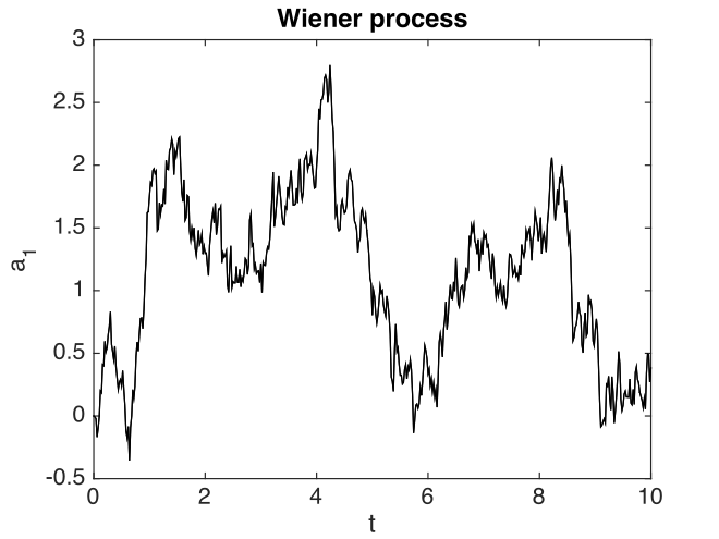
Fig. 7 Increasing the Wiener process resolution and adding a header.

Exercise

Add 100 samples and 100 serial ensemble trajectories. Does the mean equal zero within the sampling error bars?

Harmonic oscillator

The next example is the stochastic harmonic oscillator with the initial condition that

\[a(0) = 1+v,\]

where

\[\left\langle v^{2}\right\rangle = 1\]

and the differential equation:

\[\dot{a}=ia+w(t).\]

Initial conditions and derivative

First, make sure you type clear to clear the previous example. This is good practice for all the examples. The following parameters are needed to specify the harmonic oscillator with noise. By specifying return values in square brackets, the data is made available in the user data space:

clear
in.initial = @(rv,~) 1+rv;
in.ensembles = [20,20];
in.da = @(a,w,~) i*a + w;
in.olabels = {'<a_1>'};
xspde(in);

Here ~ indicates an unused input to a function, while i is the Matlab codes for the unit imaginary number, \(i\). The following graph is produced:

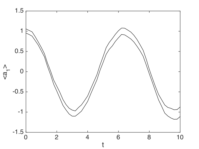
Fig. 8 Simple harmonic oscillator amplitude

The plotted error-bars are suppressed, as they are too small to see, nor is there any header, since none was specified. The xsim() program reports the following error summary, using the default number of points (51):

- Max sampling error = 1.193890e-01
- Max step error = 1.270917e-02

This is an approximate upper bound on the overall integration error of the specified observable. It is calculated from comparing two solutions. In this case, the default estimates are obtained by comparing a coarse and fine step calculation at half the specified step-size. This is used to extrapolate to zero step-size. The difference between the fine result and the extrapolated result gives the error estimate.

Comparisons with exact results

The stochastic equation has the mean solution:

\[\begin{split}\begin{aligned} \left\langle a\left(t\right)\right\rangle & = e^{it}\\ & = \cos\left(t\right)+i\sin\left(t\right) \end{aligned}\end{split}\]

To compare the calculated solution with this exact result, just tell the graphics program that you want a comparison, by editing the project file, and adding a comparison function.

This example uses the previous inputs, together with the comparison function itself (compare). All functions and data relating to observables are cell arrays, hence the curly brackets: compare{1} is the first element of an array of comparison functions that might be needed if there are many observables.

in.compare{1} = @(t,~) cos(t);
xspde(in);

With this input, xgraph gives the difference in the comparison as:

-  Maximum comparison differences = 1.950535e-01

The actual error in this case is smaller than the error estimated using the sampling error estimates. However, the error-bars are very small. This is because in this case, the specified fine step-size is small enough to give excellent convergence.

Comparison graphs are also produced, including one of the relative errors:

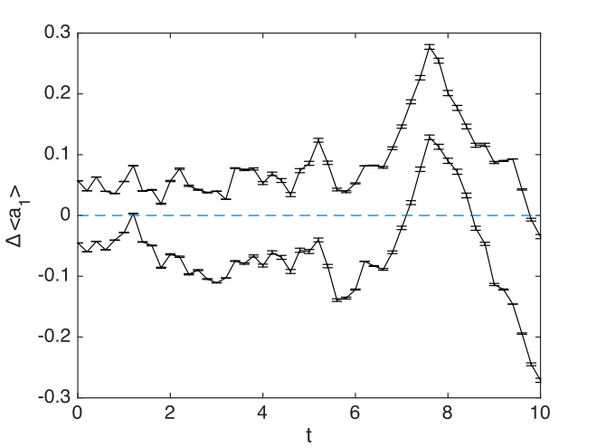
Fig. 9 Simple harmonic oscillator comparison graph: exact vs computed, with error-bars.

The reported summary data is consistent with the graphs, as expected. Note that one can obtain exactly the same result in the interaction picture, by using an imaginary linear coupling of \(i\), and a derivative term of zero. The code then reports a maximum step-size error of around \(\sim10^{-15}\), equal to the limit of IEEE arithmetic.

Exercise

Add a linear decay of \(-a\) to the differential equation, and modify the exact solution to suit, then replot. Is it exactly as you expected?

Kubo oscillator

The next example is more interesting. It is the Kubo oscillator, an oscillator with a random frequency. It is a case of multiplicative noise, but with a complex variable.

In Stratonovich stochastic calculus, its equation is:

\[\dot{a}=ia\zeta(t)\]

Given the initial condition that \(a(0)=1\), each trajectory has the solution:

\[a\left(t\right)=e^{iw(t)}\]

where

\[w(t)=\int_{0}^{t}\zeta(\tau)d\tau\]

The corresponding mean value is different to the instantaneous trajectory, owing to dephasing:

\[\left\langle a\left(t\right)\right\rangle =e^{-\left\langle w^{2}(t)\right\rangle /2}=e^{-t/2}.\]

Kubo initial conditions and derivative

Here more parameters are needed. One real noise term is required per integration point, specified using noises. Next, the ensemble numbers are required. Here we use 100 vector-level trajectories, and 16 sets at a higher level. In these calculations, the mean amplitude is calculated, and compared against a comparison function.

function e = Kubo()
    in.name = 'Kubo oscillator';
    in.ensembles = [400,16,1];
    in.initial = @(rv,r) 1+0*rv;
    in.da = @(a,w,r) i*w.*a;
    in.olabels = {'<a_1>'};
    in.compare{1} = @(t,~) exp(-t/2);
    e = xspde(in);
end

Kubo error results are reported as:

-  Max sampling error = 1.065936e-02
-  Max step error = 5.072889e-04
-  Max comparison difference = 1.269069e-02

Note that these are generally consistent with the graphs below, as they should be.

Is the actual error always less than the reported maximum standard deviation? This is not always the case, for statistical reasons. The statistical estimates given are best estimates of the standard deviations of the plotted means. However, given a large enough number of means at different times, some must fall outside the range of a unit standard deviation.

The different time points in the Kubo oscillator trajectories become uncorrelated after a time of order one. Hence an occasional excursion with an error of \(2\sigma\) can occur. In other words, the expected maximum sampling error is a multiple of the standard deviation, which should therefore be treated with some caution as a guide to statistical errors.

We see evidence here the sampling errors often exceed the step-size errors, unless large sample numbers are used.

Kubo graphs

The Graphics program reports the following errors when making the comparisons:

-  Max difference in 1 = 1.294696e-02

With this choice of algorithm and step-size, the results of a simulation run are plotted below.

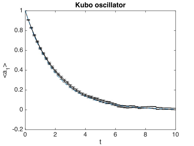
Fig. 10 Kubo oscillator mean amplitude

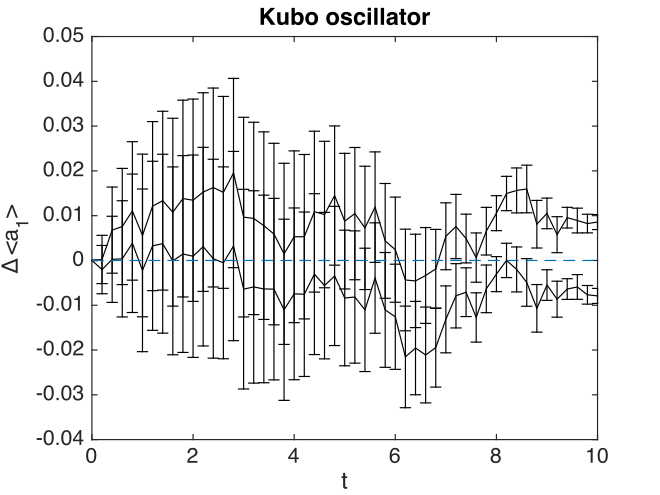
Fig. 11 Kubo oscillator amplitude errors

There are some interesting features here. The two solid lines indicate the sampling error. The error bars indicate the step-size error. This affects both results, but is only visible in the error graphs, which have an expanded scale.

Exercise

Add a detuning of \(ia\) to the differential equation, modify the exact solution to suit, then replot.

Soliton

The third example is the soliton equation for the nonlinear Schrödinger equation, with:

\[\frac{da}{dt}=\frac{i}{2}\left[\nabla^{2}a-a\right]+ia\left|a\right|^{2}\]

Together with the initial condition that \(a(0,x)=sech(x)\), this has an exact solution that doesn’t change in time:

\[a(t,x) = sech(x)\]

The Fourier transform at \(k=0\) is simply:

\[\tilde{a}(t,0) = \frac{1}{\sqrt{2\pi}}\int sech(x)dx=\sqrt{\frac{\pi}{2}}\]

Soliton parameters and functions

The important parameters and functions in this case are:

function [e] = Soliton()
    in.name = 'NLS soliton';
    in.dimension = 2;
    in.initial = @(v,r) sech(r.x);
    in.da = @(a,~,r) i*a.*(conj(a).*a);
    in.linear = @(r) 0.5*i*(r.Dx.^2-1.0);
    in.olabels = {'a_1(x)'};
    in.compare{1}= @(t,~) 1;
    e = xspde(in);
end

The xspde program reports the following maximum errors:

-  Max step error = 6.270515e-04

The output reflects the known analytic result.

Soliton graphs and errors

Graphs of results are given below.

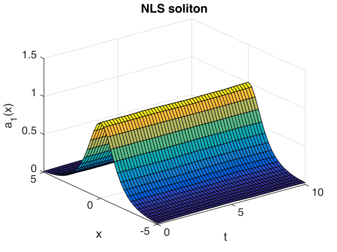
Fig. 12 Soliton amplitude versus space and time

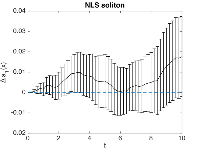
Fig. 13 Soliton amplitude errors at center

The xgraph program reports that comparison errors are slightly less than the step error:

-  Max difference in 1 = 7.875209e-03

This is not always the case, because the error checking does not check errors due to the lattice sizes. In general this needs to be carried out manually.

Exercise

Add an additive complex noise of \(0.01(dw_{1}+idw_{2}\)) to the differential equation, then replot with an average over 1000 samples.

Gaussian with HDF5 files

The fifth example is free diffraction of a Gaussian wave-function in three dimensions, given by

\[\frac{da}{dt}=\frac{i}{2}\nabla^{2}a\]

Together with the initial condition that \(a(0,x)=exp(-\left|\mathbf{x}\right|^{2}/2)\), this has an exact solution for the diffracted intensity in either ordinary space or momentum space:

\[\begin{split}\begin{aligned} \left|a\left(t,\mathbf{x}\right)\right|^{2} & = \frac{1}{\left(1+t^{2}\right)^{3/2}}exp(-\left|\mathbf{x}\right|^{2}/\left(1+t^{2}\right))\\ \left|\tilde{a}\left(t,\mathbf{k}\right)\right|^{2} & = exp(-\left|\mathbf{k}\right|^{2})\end{aligned}\end{split}\]

Gaussian inputs

Before running this simulation, be careful to change the Matlab working directory to your intended working directory, which must have write permission enabled. For example, type:

cd ~

A possible user set of parameters to simulate this is:

function [e] = Gaussian()
    in.dimension = 4;
    in.initial = @(~,r) exp(-0.5*(r.x.^2+r.y.^2+r.z.^2));
    in.da = @(a,~,~) zeros(size(a));
    in.linear = @(r) 1i*0.05*(r.Dx.^2+r.Dy.^2+r.Dz.^2);
    in.observe = {@(a,~) a.*conj(a)};
    in.olabels = '|a(x)|^2';
    in.file = 'Gaussian.h5';
    in.images = 4;
    in.imagetype = 1;
    in.transverse = 2;
    in.headers = 1;
    in.compare{1} = @(t,~) [1+(t/10).^2].^(-3/2);
    [e,in] = xsim(in);
    e = e+xgraph(in.file);
end

Here the program writes an HDF5 data file using xsim(), and then reads it in with the stored file-name, using xgraph(). Note that xsim() may have to change the file-name to avoid overwriting any old data. In this case, it returns the new file-name is uses. The program reports the following maximum step-size errors, which in this case are negligible, as they are purely due to the interaction picture transformations:

-  Max step error = 4.107825e-15

However, the finite spatial lattice size introduces errors in the on axis intensity, in coordinate space. This shows up in the comparisons:

-  Max difference in 1 = 5.590272e-07

Gaussian graphs

With this choice of algorithm and step-size, the results of a simulation run are plotted below. The errors, of order \(10^{-7}\), are simply due to interference of diffracted waves caused by the periodic boundary conditions. This is sometimes called aliasing error. One can think of this physically as being a simulation of an infinite array or periodically repeated Gaussian inputs, which can diffract and interfere.

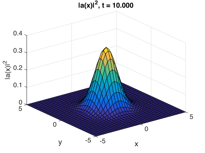
Fig. 14 Image of transverse gaussian intensity at \(t=0\).

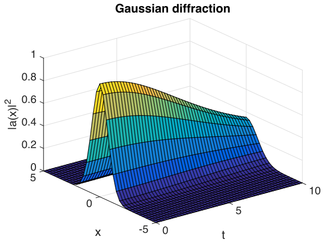
Fig. 15 Gaussian intensity diffraction

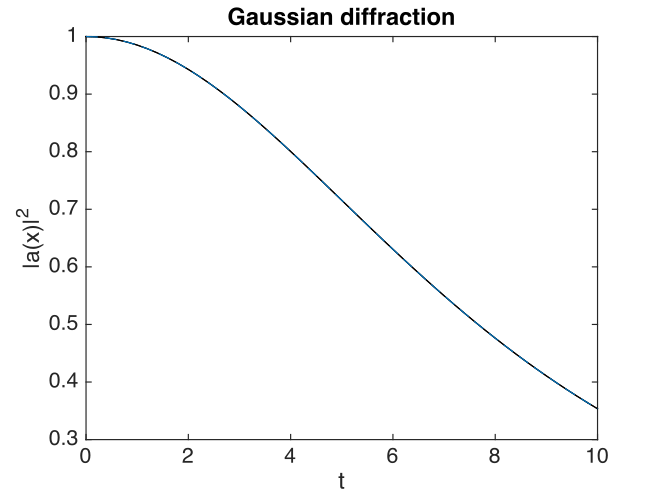
Fig. 16 Gaussian intensity at \(\boldsymbol{r}=0\).

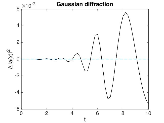
Fig. 17 Gaussian, modulus-squared errors at \(\boldsymbol{r}=0\) .

Exercise

Add an additive complex noise of \(0.01(dw_{1}+idw_{2}\)) to the Gaussian differential equation, then replot with an average over 10 samples.

Planar noise

The fifth example is growth of thermal noise of a two-component complex field in a plane, given by the equation

\[\frac{d\boldsymbol{a}}{dt}=\frac{i}{2}\nabla^{2}\boldsymbol{a}+\boldsymbol{\zeta}(t,x)\]

where \(\boldsymbol{\zeta}\) is a delta-correlated complex noise vector field:

\[\zeta_{j}(t,\mathbf{x})=\left[\zeta_{j}^{re}(t,\mathbf{x})+i\zeta_{j}^{im}(t,\mathbf{x})\right]/\sqrt{2},\]

with the initial condition that the initial noise is delta-correlated in position space

\[a(0,\mathbf{x})=\boldsymbol{\zeta}^{(in)}(\boldsymbol{x})\]

where:

\[\boldsymbol{\zeta}^{(in)}(\boldsymbol{x})=\left[\boldsymbol{\zeta}^{re(in)}(\mathbf{x})+i\boldsymbol{\zeta}^{im(in)}(\mathbf{x})\right]/\sqrt{2}\]

This has an exact solution for the noise intensity in either ordinary space or momentum space:

\[\begin{split}\begin{aligned} \left\langle \left|a_{j}\left(t,\mathbf{x}\right)\right|^{2}\right\rangle & = (1+t)/\Delta V\\ \left\langle \left|\tilde{a}_{j}\left(t,\mathbf{k}\right)\right|^{2}\right\rangle & = (1+t)/\Delta V_{k}\\ \left\langle \tilde{a}_{1}\left(t,\mathbf{k}\right)\tilde{a}_{2}^{*}\left(t,\mathbf{k}\right)\right\rangle & = 0 \end{aligned}\end{split}\]

Here, the noise is delta-correlated, and \(\Delta V\), \(\Delta V_{k}\) are the cartesian space and momentum space lattice cell volumes respectively. Suppose that \(N=N_{x}N_{y}\) is the total number of spatial points, and \(V=R_{x}R_{y}\), where there are \(N_{x(y)}\) points in the x(y)-direction, with a total range of \(R_{x(y)}\). Then, \(\Delta x=R_{x}/N_{x}\) ,\(\Delta k_{x}=2\pi/R_{x}\) , so that:

\[\begin{split}\begin{aligned} \Delta V & = \Delta x\Delta y=\frac{V}{N}\\ \Delta V_{k} & = \Delta k_{x}\Delta k_{y}=\frac{(2\pi)^{2}}{V}. \end{aligned}\end{split}\]

In the simulations, two planar noise fields are propagated, one using noise generated in position space, the other with noise generated in momentum space. This example shows that, provided no filters are applied, both types of noise are identical in their effects. However, momentum space noise requires an N-dimensional inverse FFT before being added, which is slower, so this method is not recommended unless needed.

Planar inputs

function [e] = Planar()
    in.name = 'Planar noise growth';
    in.dimension = 3;
    in.fields = 2;
    in.ranges = [1,5,5];
    in.steps = 2;
    in.noises = [2,2];
    in.ensembles = [10,2,2];
    in.initial = @Initial;
    in.da = @D_planar;
    in.linear = @Linear;
    in.observe{1} = @(a,r) xint(a(1,:).*conj(a(1,:)),r);
    in.observe{2} = @(a,r) xint(a(2,:).*conj(a(2,:)),r.dk,r);
    in.observe{3} = @(a,r) xave(a(1,:).*conj(a(2,:)));
    in.transforms = {[0,0,0],[0,1,1],[0,1,1]};
    in.olabels{1} = '<\int|a_1(x)|^2 d^2x>';
    in.olabels{2} = '<\int|a_2(k)|^2 d^2k>';
    in.olabels{3} = '<‌<a_1(k)a^*_2(k)>‌>';
    in.compare{1} = @(t,in) [1+t]*in.nspace;
    in.compare{2} = @(t,in) [1+t]*in.nspace;
    in.compare{3} = @(t,in) 0;
    in.images = [4,2,0];
    in.transverse = [2,2,0];
    in.pdimension = [4,1,1];
    e = xspde(in);
end
function a0 = Initial(v,r)
    a0(1,:)  = (v(1,:)+1i*v(2,:))/sqrt(2);
    a0(2,:)  = (v(3,:)+1i*v(4,:))/sqrt(2);
end
function da = D_planar(a,w,r)
    da(1,:)  = (w(1,:)+1i*w(2,:))/sqrt(2);
    da(2,:)  = (w(3,:)+1i*w(4,:))/sqrt(2);
    end
function L = Linear(r)
    lap = r.Dx.^2+r.Dy.^2;
    L(1,:)  = 1i*0.5*lap(:);
    L(2,:)  = 1i*0.5*lap(:);
end

Planar graphs

With this choice of algorithm and step-size, the results are plotted below.

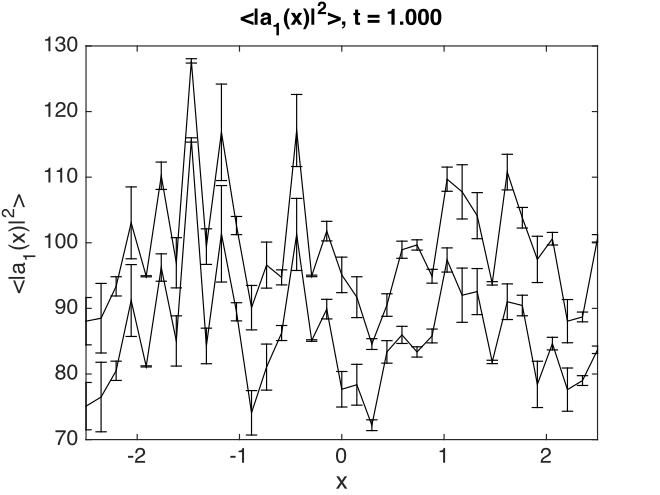
Fig. 18 Planar noise intensity as a transverse slice in the \(t=1\), \(y=0\) plane. The relatively large sampling error is because there are not many samples.

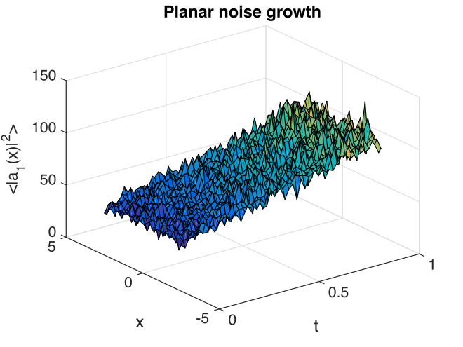
Fig. 19 Growth in noise intensity with time vs. \(x\), at \(y=0\).

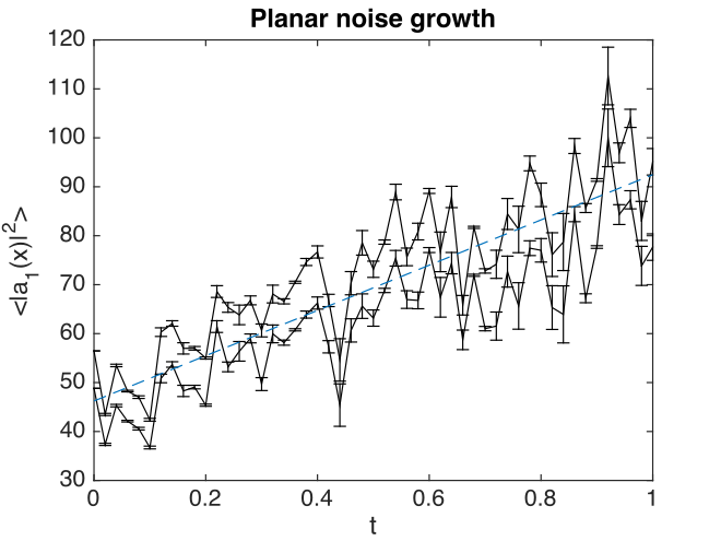
Fig. 20 Growth in planar noise intensity at \(x=y=0\), vs. exact results.

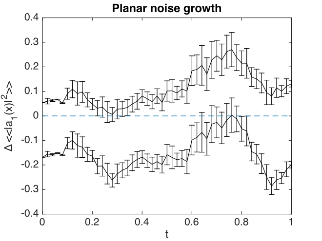
Fig. 21 Errors in planar noise intensity at \(x=y=0\), vs. exact results. These results are averaged across the plane, as well as being ensemble averaged.

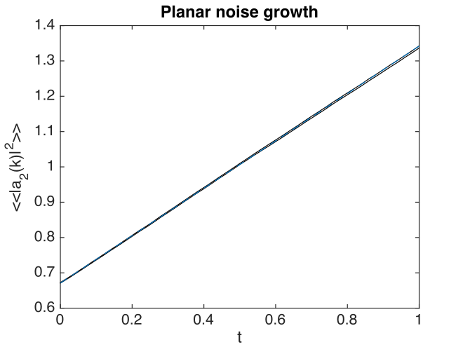
Fig. 22 Growth in planar noise intensity in momentum space, for the second field, at \(k_{x}=k_{y}=0\).

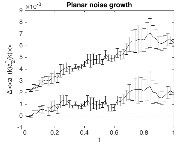
Fig. 23 Lattice averaged errors in cross-correlations in momentum space, vs. exact results.

Exercise

Add a decay rate of \(-a\) to the Planar differential equation, then replot.

Extensible simulations

Next, an extensible simulation: first a noisy absorber, then a noisy amplifier. The second part has a different differential equation, and larger graphical scales.

This is handled with the extensibility feature of xSPDE. Just enter a sequence of inputs, in the form {in1, in2, in3, ...} with a corresponding sequence of graphs, {g1, g2, g3m ...}. Here, the first equation is:

\[\frac{da}{dt}=-a+\zeta_{1}(t)+i\zeta_{2}(t)\]

with an initial condition of \(a=1\). The mean intensity is constant:

\[\left\langle \left|a(t)\right|^{2}\right\rangle = 1.\]

Input file

The full input file is given below.

function [e] = Gain()
    in.name = 'Loss with noise';
    in.ranges = 4;
    in.noises = [2,0];
    in.ensembles = [100,16,1];
    in.initial = @(v,~) (v(1,:)+1i*v(2,:))/sqrt(2);
    in.da = @(a,w,r) -a + w(1,:)+1i*w(2,:);
    in.observe{1} = @(a,~,~) a.*conj(a);
    in.olabels = {'|a|^2'};
    in.compare = {@(t,~) 1+0*t};
    in2 = in;
    in2.steps = 4;
    in2.origin = in.ranges;
    in2.name = 'Gain with noise';
    in2.da = @(a,z,r) a + z(1,:)+1i*z(2,:);
    in2.compare = {@(t,~) 2*exp(2*(t-4))-1};
    e = xspde({in,in2});
end

Note that the code defines in2 = in before making any changes, so that only a few additional inputs are needed. The number of steps is increased to improve the accuracy of the second integration, and the second time origin is chosen so that it starts from the time the first simulation is completed.

Results are graphed below.

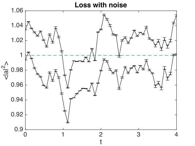
Fig. 24 Absorber intensity

Comparison graphs are also produced for the relative errors. In the graph given here,

Extended simulations

The second differential equation has an initial condition corresponding to the solution of the first equation at \(t=4\), and the derivative:

\[\frac{da}{dt}=a+\zeta_{1}(t)+i\zeta_{2}(t)\]

The mean intensity grows exponentially:

\[\left\langle \left|a\right|^{2}\right\rangle =1.\]

\[ \begin{align}\begin{aligned} \left\langle \left|a(t)\right|^{2}\right\rangle =2e^{2(t-4)}-1\\where\end{aligned}\end{align} \]

\[w(t)=\int_{0}^{t}\zeta(t^\prime)dt^\prime\]

To compare the calculated solution with this exact result, there are two compare functions in the project file. The time axis in the second graph has the origin reset to zero.

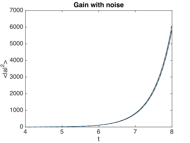
Fig. 25 Noisy amplifier intensity

Comparison graphs of the relative errors are also produced here as well.

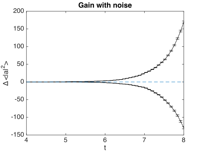
Fig. 26 Noisy amplifier intensity errors, showing how the sampling errors increase in time.

Exercise

Reverse the order of gain and loss.

Characteristic

The next example is the characteristic equation for a traveling wave at constant velocity,

\[\frac{da}{dt}+\frac{da}{dx}=0\]

Together with the initial condition that \(a(0,x)=sech(2x+5)\), this has an exact solution that propagates at a constant velocity:

\[a(t,x) = sech(2(x-t)+5)\]

The time evolution at \(x=0\) is simply:

\[a(t,0) = sech(2(t-5/2))\]

Characteristic inputs

The important parameters and functions in this case are:

function [e] = Characteristic()
    in.name = 'Characteristic'
    in.dimension = 2;
    in.initial = @(~,r) sech(2.*(r.x+2.5));
    in.da = @(a,~,r) 0*a;
    in.linear = @(r) -r.Dx;
    in.olabels = {'a_1(x)'};
    in.compare = {@(t,in) sech(2.*(t-2.5))};
    e = xspde(in);
end

The simulation program reports the following maximum errors:

-  Max step error = 5.773160e-15

This is slightly misleading, since while the interaction picture is essentially exact, it is solving a finite lattice problem exactly. The transverse lattice discretization does introduce errors of course, and these are seen in the comparisons with the exact results:

-  Maximum comparison differences = 7.581817e-03

Graphs of results are given below.

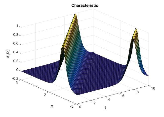
Fig. 27 Characteristic traveling wave versus space and time

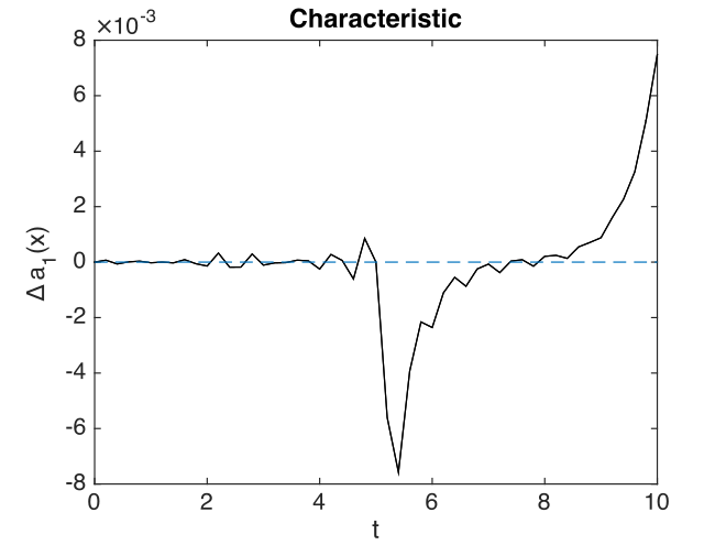
Fig. 28 Characteristic errors at center

Exercise

Recalculate with the opposite velocity, and a new exact solution.

Equilibrium

We now move on to frequency space simulations. The equation is the same as the earlier loss equation, that is

\[\frac{da}{dt}=-a+\zeta(t)\]

where \(\zeta(t)=\zeta_{1}(t)+i\zeta_{2}(t)\), with an initial condition of \(a=(w_{1}+iw_{2})/\sqrt{2}\). For sufficiently long time-intervals, the solution is given by:

\[\tilde{a}\left(\omega\right)=\frac{\tilde{\zeta}(\omega)}{1-i\omega}\]

The expectation value of the noise Fourier transform modulus squared, in the large \(T\) limit, is therefore:

\[\begin{split}\begin{aligned} \left\langle \left|\tilde{a}(\omega)\right|^{2}\right\rangle & = \frac{1}{2\pi\left(1+\omega^{2}\right)}\int\int e^{i\omega(t-t')}\left\langle \zeta(t)\zeta^{*}(t')\right\rangle dtdt'\,.\\ & = \frac{T}{\pi\left(1+\omega^{2}\right)}\end{aligned}\end{split}\]

Program inputs

The full input file is given below.

function e = Equilibrium()
    in.name = 'Equilibrium spectrum';
    in.points = 640;
    in.ranges = 100;
    in.noises = [2,0];
    in.ensembles = [100,1,10];
    in.initial = @(v,~) (v(1,:)+1i*v(2,:))/sqrt(2);
    in.da = @(a,z,r) -a + z(1,:)+1i*z(2,:);
    in.observe{1} =@(a,~) a.*conj(a);
    in.observe{2} =@(a,~) a.*conj(a);
    in.transforms ={0,1};
    in.olabels = {'|a(t)|^2', '|a(w)|^2'};
    in.compare = {@(t,~) 1.+0*t, @(w,~)100.16./(pi*(1+w.^2))};
    e = xspde(in);
end

Results are graphed below. The calculated spectrum is indistinguishable from the exact result.

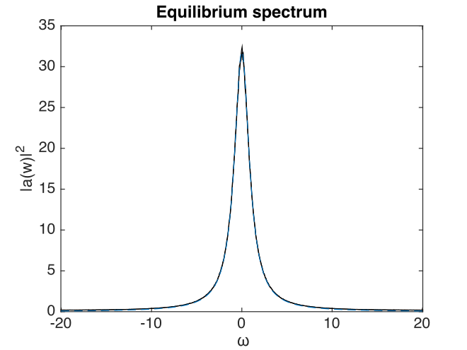
Fig. 29 Equilibrium spectral intensity

The xsim program reports the following error summary:

-  Max step error = 5.856892e-02
-  Max sampling error = 4.234763e-01
-  Maximum comparison differences = 6.194415e-01

Here, the comparison differences indicate that the maximum error reported is actually about 1.5 standard deviations of the maximum sampling error. Given the large number of data points, this is a reasonable result.

Exercise

Add a second field coupled to the first, so that:

\[\begin{split}\begin{aligned} \frac{da}{dt} & = -a+\zeta(t)\\ \frac{db}{dt} & = -b+a \end{aligned}\end{split}\]

Compare the two spectra, and calculate what the second one should look like.