Interactive xSPDE
All xSPDE simulations require parameters stored in an input structure used by the xSPDE toolbox. Inputs have default values, which can be changed by creating fields in the input structure. A complete list of parameters and their uses is given in Public API.
The simplest way to use xSPDE is via the interactive Matlab command window, illustrated in this chapter. In this mode of operation, any required parameters are entered into the input structure in, and then the command xspde(in) runs and graphs the simulation.
Note that one must enter clear first to erase previous data in the Matlab workspace, unless the previous data is being recycled.
Stochastic equations
An ordinary stochastic equation [Kloeden1995] for a real or complex vector \(\boldsymbol{a}\) is:
Here \(\boldsymbol{A}\) is a vector function, \(\underline{\mathbf{B}}\) a matrix, and \(\boldsymbol{\zeta}\) is a real Gaussian distributed noise vector such that \(\left\langle \boldsymbol{\zeta}\right\rangle = 0\), and :
To simulate a stochastic equation like this interactively, first make sure Matlab path is pointing to the xSPDE folder and type clear to clear old data.
Next, enter the xspde parameters (see Public API) into the command window, as follows:
in.label1 = <parameter1>
in.label2 = ...
in.da = @(a,w,r) <expression for da/dt>
xspde(in)
- The notation
in.label = parametercreates a field in the structurein(which is created dynamically, if it has not been defined before). - The notation
@(..)is the Matlab shorthand for an anonymous function. - The parameters passed to the
da()function are:a, the stochastic variable;w, the random noise; andr, the input structure with additional coordinates and parameters. xspde()is called with the input structure as the only argument.- parameters or functions that are omitted are replaced with default values.
- a sequence of simulations requires an input list: {in1,in2..}.
Once the simulation is completed, xSPDE will generate graphs of averages of any required observables or moments. If needed, simulated data is stored in specified files for later use, which requires a file-name to be entered.
Interactive examples
The random walk
The first example is the simplest possible stochastic equation:
with a complete xSPDE script in Matlab below, and output in Fig. 1.
in.da = @(a,w,r) w; xspde(in);
- Here
da()defines the derivative function, withwbeing the noise. - The last argument of xspde user functions is
r, containing the parameters required for the simulation.
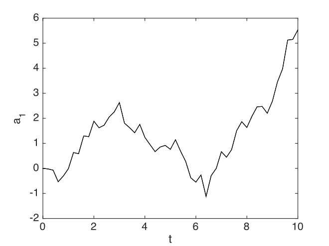
Fig. 1 The simplest case: a random walk.
Laser quantum noise
Next we treat a model for the quantum noise of a single mode laser:
where \(\zeta=\left(w_{1}+iw_{2}\right)\), so that:
Here the coefficient \(b\) describes the quantum noise of the laser, and is inversely proportional to the equilibrium photon number. An xSPDE script in Matlab is given below, for the case of \(b=0.01\), with an output graph in Fig. 2. Note the use of the clear command here to clean up the Matlab workspace before the start.
clear
in.noises = 2;
in.observe = @(a,r) abs(a)^2;
in.olabels = '|a|^2';
in.da = @(a,w,r) (1-abs(a)^2).*a+0.01*(w(1)+i*w(2));
xspde(in)
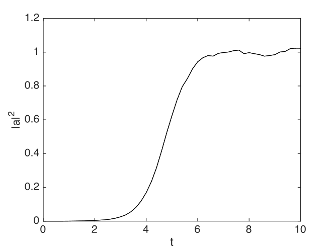
Fig. 2 Simulation of the stochastic equation describing a laser turning on.
Note that:
Ito and Stratonovich equations
The xSPDE toolbox is primarily designed to treat Stratonovich equations [Gardiner2004], which are the broad-band limit of a finite band-width random noise equation, with derivatives evaluated at the midpoint in time of a time-step.
An equivalent type of stochastic equation is the Ito form. This is written in a similar way to a Stratonovich equation, except that this corresponds to a limit where derivatives are evaluated at the start of each step. To avoid confusion, we can write an Ito equation as a difference equation:
Here:
When \(\mathbf{\mathsf{B}}\) is not a constant, the Ito drift term is different to the Stratonovich one. This difference occurs because the noise term is non-differentiable. The relationship is that
Provided the noise coefficient \(B\) is constant - which is called additive noise - there is no real difference between the two types of equation. Otherwise, it is essential to know which type of stochastic equation it is, in order to get unambiguous results!
Financial calculus
The Black-Scholes equation is a well-known Ito stochastic equation, used to price financial options. It describes the fluctuations in a stock value:
where \(\left\langle dw^{2}\right\rangle =dt\). Since the noise is multiplicative, the equation is different in Ito and Stratonovich forms of stochastic calculus. The corresponding Stratonovich equation, as used in xSPDE is:
An interactive xSPDE script in Matlab is given below with an output graph in Fig. 3, for the case of a volatile stock with \(\mu=0.1\), \(\sigma=1\). Note the spiky behaviour, typical of multiplicative noise, and also of the risky stocks in the small capitalization portions of the stock market.
clear
in.initial = @(rv,r) 1;
in.da = @(a,w,r) -0.4*a+a*w;
xspde(in)
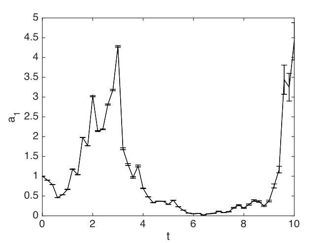
Fig. 3 Simulation of the Black-Scholes equation describing stock prices.
- Here
initial()describes the initialization function. - The first argument of
@(v,r)isv, an initial random variable. - The error-bars are estimates of step-size error.
- Errors can be reduced by using more time-steps: see Averaging and projects.
This graph is of a single stochastic realisation. Generation of averages is also straightforward. This is described in Averaging and projects.
Stochastic partial differential equations
More generally, xSPDE solves [Werner1997] a stochastic partial differential equation for a complex vector field defined with arbitrary transverse dimension. The total dimension is then input as \(d=2,3,...\). Equations of this type occur in many disciplines, including biology, chemistry, engineering and physics. They are in differential form as
Here \(\boldsymbol{a}\) is a real or complex vector or vector field. The initial conditions are arbitrary functions. \(\boldsymbol{A}\left[\boldsymbol{a}\right]\) and \(\underline{\mathbf{B}}\left[\boldsymbol{a}\right]\) are vector and matrix functions of \(\boldsymbol{a}\), \(\underline{\mathbf{L}}\left[\boldsymbol{\nabla}\right]\) is a matrix of linear terms and derivatives, diagonal in the vector indices, and \(\mathbf{\boldsymbol{\zeta}}=\left[\boldsymbol{\zeta}^{x},\boldsymbol{\zeta}^{k}\right]\) are real delta-correlated noise fields such that:
Note that the x and k noise term for each value of the index are generated from the same underlying stochastic process. This is necessary because there are some equations that require both a filtered and unfiltered noise generated from the same underlying random number distribution. If these correlations are not wanted, and the noises are required to be independent, then different noise indices must be used.
Transverse boundary conditions are assumed periodic as the default option, which allows the use of efficient spectral Fourier transform propagation codes. Other types of boundary conditions available are Neumann boundaries with zero normal derivatives, and Dirichlet boundaries with zero fields at the boundary. These require the use of finite difference methods. The boundary type can be individually specified in each axis direction. The term \(\underline{\mathbf{L}}\left[\boldsymbol{\nabla}\right]\) may be omitted, as space derivatives can also be treated directly in the derivative function, and this is necessary with Neumann or Dirichlet boundaries. The momentum filter \(f(\boldsymbol{k})\) is an arbitrary user-specified function, allowing for spatially correlated noise.
To treat stochastic partial differential equations or SPDEs, the equations are divided into the first two terms, which are essentially an ordinary stochastic equation, and the last term which gives a linear partial differential equation:
The interaction picture is a moving reference frame used to solve the linear part of the equation exactly, defined by an exponential transformation. This is carried out internally by matrix multiplications and Fourier transforms.
In more detail, in Fourier space, if \(\tilde{\boldsymbol{a}}\left(\boldsymbol{k}\right)=\mathcal{F}\left[\boldsymbol{a}\left(\mathbf{x}\right)\right]\) is the Fourier transform of \(\boldsymbol{a}\), we simply define:
where the propagation function can be written intuitively as \(\mathcal{P}=\exp\left[\underline{\mathbf{L}}(\mathbf{D})dt\right]\), where \(\mathbf{D}=i\boldsymbol{k}\sim\nabla\). The function \(\underline{\mathbf{L}}(\mathbf{D})\) is input using the xSPDE linear response function linear(). With this definition, at each step the equation that is solved can be re-written in a more readily soluble form as:
The total derivative in the interaction picture is the xSPDE derivative function da():
where usually \(\boldsymbol{A}\), \(\underline{\mathbf{B}}\) are evaluated at the midpoint which is the origin in the interaction picture. For convenience, the final output is calculated in the original picture, with at least two interaction picture (IP) transformations per time-step.
Note that there are many types of partial differential equation that can be treated with xSPDE, even if the interaction picture method doesn’t apply. This occurs when there are nonlinear functions with arbitrary derivatives, or derivatives that are non-diagonal in the vector indices. For these cases, the space derivatives are evaluated inside the derivative term da():. If there are higher order time derivatives as well, these can be re-expressed as a set of first-order time derivatives, provided the problem is an initial-value problem.
Symmetry breaking
An example of a SPDE with space-time dimensions of \(d=3\) is the stochastic Ginzburg-Landau equation. This describes symmetry breaking, in which the system develops a spontaneous phase which can vary spatially. The model is widely used in fields ranging from lasers to magnetism, superconductivity, superfluidity and even particle physics:
where
An xSPDE script is given below, for parameter values of \(b=0.001\) and \(c=0.01\), with the output graphed in Fig. 4. Note that in the graph, the range -5<x<5 is the default xSPDE coordinate range, while
the .* notation is used in functions here, as fields require element-wise multiplication.
clear
in.noises = 2;
in.dimension = 3;
in.steps = 10;
in.linear = @(r) i*0.01*(r.Dx.^2+r.Dy.^2);
in.observe = @(a,~) abs(a).^2;
in.olabels = '|a|^2';
in.da = @(a,w,~) (1-abs(a(1,:)).^2).*a+0.001*(w(1,:)+i*w(2,:));
xspde(in)
Here:
dimensionis the space-time dimension, with an \(x-t\) plot given here.stepsgives the integration steps per plot-point, for improved accuracy.linearis the linear operator — an imaginary laplacianr.Dxindicates a derivative operation, \(\partial/\partial x\). See the reference entry forlinearfor more information.
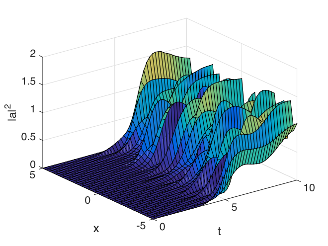
Fig. 4 Simulation of the stochastic equation describing symmetry breaking in two dimensions. Spatial fluctuations are caused by the different phase-domains that interfere. The graph obtained here is projected onto the \(y=0\) plane.