Averaging and projects
Using xsim and xgraph
Suppose that you are not happy with the graphs in an interactive session, and want to alter them by adding a heading or some other change. For long simulations, it may be inconvenient to re-run everything. This is easy, provided the data is in the current workspace.
For example, suppose the Kubo simulation is run interactively, using an output specification so that the data file is stored locally in your Matlab workspace. After editing some inputs, the job can be repeated, with data saved to the local workspace, by running
[e,data] = xspde(in)
Alternatively, if you just want the data, and no graphs, use:
[e,input,data] = xsim(in)
Next, you should know the object label you wish to change. Note that the xsim() and xgraph() program inputs are either structure objects containing data for one simulation, or else cell arrays of structures with many simulations in sequence, which are treated later. You can use
either in xSPDE.
To change the project name for the graph headings, input:
in.name ='My new project';
then replot the data using
xgraph(data,in)
More graphics information can be added, for example using
in.olabels = 'Intensity';
which inputs this additional graphics data to the in structure to xSPDE. Just plot again, using the same instructions.
Ensembles in xSPDE
Averages over stochastic ensembles are the specialty of xSPDE, which requires specification of the ensemble size. To get an average, an ensemble size is needed, to obtain more trajectories in parallel.
Ensembles are specified in three levels to allow maximum resource utilization, so that:
in.ensembles = [ensembles(1), ensembles(2), ensembles(3)]
The first, ensembles(1), gives within-thread parallelism, allowing vector instruction use for single-core efficiency. The second, ensembles(2), gives a number of independent trajectories calculated serially.
The third, ensembles(3), gives multi-core parallelism, and requires the Matlab parallel toolbox. This improves speed when there are multiple cores, and one should optimally put ensembles(3) equal to the available number of CPU cores.
The total number of stochastic trajectories or samples is ensembles(1) * ensembles(2) * ensembles(3).
However, either ensembles(2) or ensembles(3) are required if sampling error-bars are to be calculated, owing to the sub-ensemble averaging method used in xSPDE to calculate sampling errors
accurately.
Random walk with averaging
To demonstrate this, try adding some more trajectories, points and an output label to the in parameters of the random walk example:
- ::
- clear in.da = @(a,w,r) w; in.ensembles = [500,20]; in.points = 101; in.olabels = ‘<a_1>’; xspde(in)
You will see Fig. 5 appearing.
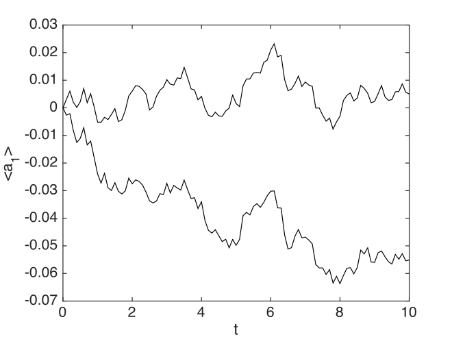
Fig. 5 The average random walk with \(10^{4}\) trajectories.
This looks like the earlier graph, but check the vertical scale. The in.ensembles = [100, 100] input gives an average over \(10^{4}\) random trajectories. Therefore the sampling error is accordingly reduced by a factor of 100. The two lines plotted are the upper and lower one standard deviation limits.
The more detailed structure of the random walk is due to having more time-points. Of course, \(\left\langle a\right\rangle =0\) in the ideal limit.
Note that:
xSPDE projects
An XPDE session can either run simulations interactively, described in Interactive xSPDE, or else using a function file called a project file. This allows xSPDE to run in a batch mode, as needed for longer projects which involve large ensembles. In either case, the Matlab path must include the xSPDE folder.
A minimal xSPDE project function is as follows:
function = project()
    in.label1 = parameter1;
    in.label2 = parameter2;
    ...
    xspde(in)
end
For standard graph generation, the script input or project function should end with the combined function xspde(). Alternatively, to generate simulation data and graphs separately, the function xsim() runs the simulation, and xgraph() makes the graphs. The two-stage option is better for running batch jobs, which you can graph at a later time. See the next chapter for details.
After preparing a project, type the project name into the Matlab interface, or click on the Run arrow above the editor window.
In summary:
- For medium length simulations with more control, use a function file whose last executable statement is
xspde(in).
Kubo project
To get started on more complex stochastic programs, we next simulate the Kubo oscillator, which is a stochastic equation with multiplicative noise. It uses the Stratonovich stochastic calculus. It corresponds to an oscillator with a random frequency, with difference equation:
To simulate this, one can use a file, Kubo.m, which also contains definitions of user functions.
function [e] = Kubo()
    in.name = 'Kubo oscillator';
    in.ensembles = [400,16];
    in.initial = @(rv,~) 1+0*rv;
    in.da = @(a,w,r) i*a.*w;
    in.olabels = {'<a_1>'};
    e = xspde(in);
end
The resulting graph is given in Fig. 6, including upper and lower one standard deviation sampling error limits to indicate the accuracy of the averages. This is obtained on inputting the second number in the ensembles vector, to allow sub-ensemble averaging and sampling error estimates. Note that .* multiplication must be used because the first ensemble is stored as a matrix, to improve speed.
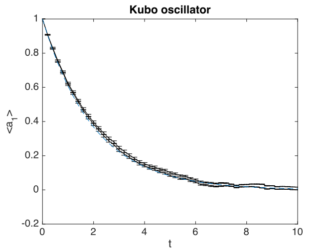
Fig. 6 The amplitude decay of a Kubo oscillator.
The other input parameters are not specified explicitly. Default values are accessed from the inpreferences function.
Here we note that:
Kubodefines the parameters and function handles, then runs the simulation.namegives a name to identify the project.ensemblesspecifies 400 samples in a parallel vector, repeated 16 times in series.initial()initializes the input to ones; the noiservis used as it has the same lattice dimension as theafield.da()is the function, \(da/dt=iaw\), that specifies the equation being integrated.olabelsis a cell array with a label for the variableathat is averaged.xspde()runs the simulation and graphics program using data from theinstructure.
The function names can point to external files instead of those in the project file itself. This is useful when dealing with complex projects, or if you just want to change one function at a time. As no points or ranges were specified, here, default values of 51 points and a range of 10 are used.
Data files and batch jobs
It is often inconvenient to work interactively, especially for large simulations. To save data is very useful. This is not automatic: to create a data file, you must enter the filename - either interactively or a bath file — before running the simulation, using the in.file = filename input.
The xSPDE program allows you to specify a file name that stores data in either standard HDF5 format, or in Matlab format. It also gives multiple ways to edit data for either simulations or graphs. A simple interactive workflow is as follows:
- Create the metadata
in, and include a file name, sayin.file = `filename.mat`. - Run the simulation with
xsim(). - Run
xgraph(`filename.mat`), and the data will be accessed and graphed.
Saving data files
In greater detail, first make sure you have a writable working directory with the command cd ~. Next, specify the filename using the in.file = 'name.ext' inputs, and run the simulation. All calculated data as well as the input metadata from the in object is stored.
For example,
in.file = 'filename.mat'
gives a Matlab data file — which is the simplest to edit.
Alternatively,
in.file = 'filename.h5'
gives an international standard HDF5 data file, useful for exchanging data with other programs.
To reload and reanalyze any previously saved Matlab simulation data, say Kubo.mat, at a later time, there are two possible approaches, described below.
Graphing saved data
If the filename is still available in an interactive session workspace, just type
xgraph(in.file)
which tells xgraph() to use the file-name already present in in.
More generally, one can use any file name directly in xgraph(), which works with either matlab or HDF5 file types. Once the data is saved in a file by running xsim() or xspde() with an input filename, just type:
xgraph('filename.mat'),
or for HDF5 files,
xgraph('filename.h5')
to replot the resulting data.
Note that you can use xgraph() with either Matlab or HDF5 file data inputs, and without having to specify the in structure. This metadata is automatically saved with the data in the output file. This approach has the advantage that many simulations can be saved and then graphed later. In the current version, in order to access the function handles in the saved files, Matlab needs to access the original input file. Hence, when you move the data to a new computer, it is best to include the original input file in the same directory as the data, to make the handles available.
Editing saved data
If the saved data was a Matlab file, one can load the simulated data and metadata by typing, for example,
load Kubo
Results can easily be replotted interactively, with changed input and new graphics details, using this method. This approach loads all the relevant saved data into your work-space.
Hence one can easily edit and change the graphics inputs in the in structure, then use the standard graphics command:
xgraph(data, in)
To change cell contents for a sequence, be aware that sequence inputs are stored in cell arrays with curly bracket indices, so you have to change them individually using an index.
Combining saved data with new metadata
If the graphs generated from saved data files need changing, some new input specifications may be needed.
To combine an old, saved data file, say 'Kubo.mat' with a new input specification in you have just created, type
xgraph('Kubo.mat', in)
or if the data was saved in an HDF5 file, it is:
xgraph('Kubo.h5', in)
In both cases the new in metadata is combined with the old metadata. Any new input metadata takes precedence over old, filed metadata.
This allows fonts and labels, for example, to be easily changed — without having to re-enter all the simulation input details.
Sequential integration
Sequences of calculations are available simply by adding a sequence of inputs to xSPDE, representing changed conditions or input/output processing. These are combined in a single file for data storage, then graphed separately. The results are calculated over specified ranges, with it’s own parameters and function handles. In the current version of xSPDE, the numbers of ensembles must be the same throughout.
The initialization routine for the first fields in the sequence is called initial(), while for subsequent initialization it is called transfer. The sequential initialization function has four input arguments, to allow noise to be combined with previous field values and input arguments, as may be required in some types of simulation. This is described in the next chapter.
In many cases, the default transfer value — which is to simply reuse the final output of the previous set of fields — is suitable. To help indicate the order of a sequence, a time origin can be included optionally with sequential plots, so that the new time is the end of the previous time, if this is required.
Suppose the project has a sequence of two simulations, with input structures of in1, in2. To run this and store the data locally, just type:
[e,~,data] = xspde({in1,in2})
To change the file headers, at a later stage, type:
in1.name = 'My first simulation'
in2.name = 'My next simulation'
This method requires that the data, in1 and in2 are already loaded into your Matlab work space so they can be edited.
Next, simply replot the data using
xgraph(data, {in1, in2})
xSPDE hints
- When using xSPDE, it is a good idea to first run the batch test script,
Batchtest.m. This will perform simulations of different types, and report an error score. The final error score ought to match the number in the script comments, to show your installation is working correctly. - xSPDE also tests your parallel toolbox installation. If you have no license for this, just omit the third ensemble setting, so that the parallel option is not used.
- To create a project file, it is often easiest to start with an existing project function with a similar equation. There are a number of these distributed with xSPDE, and these are included in the Batchtest examples.
- Just as in interactive operation, the simulation parameters and functions for a batch job are defined in the structure
in. The parameters include function handles that point to user specified functions, which give the initial values, derivative terms and quantities measured. The function handles can point to any function declarations in the same file or Matlab path. - Graphics parameters and a comparison function are also defined in the structure
in. In each case there are default parameters in a preference file, but the user inputs will be used first if included.
The general workflow is as follows:
Create a project file, using an existing example as a template
Decide whether you want to generate graphs now (xspde()) or later (xsim() and xgraph()).
Edit the project file parameters and functions
Check that the Matlab path includes the xSPDE folder
Click Run
Save the output graphs that you want to keep
More details and examples will be given in later sections!